Using Wikidata to draw networks of Politically Exposed Persons #1

Some time ago I was doing a demo for querying Politically Exposed Persons from Wikidata. This was supposed to be a part of a bigger project which didn’t materialize. Nevertheless the code can be a good exercise in the topic, so I am sharing it for anyone that might be curious.

Additionally, I wanted to do the project in python, so that finally I have enough reasons to make a demo shiny app in python (this will be in part two of this series).

Wikidata, the knowledge base maintained by Wikimedia, has a SPARQL query service. SPARQL is kind of like SQL, but not really, and it takes some time getting used to it. Fortunately, Wikidata maintains excelent documentation, as well as a point and click query builder which is quite useful.

The Wikidata query

It is possible to explore wikidata through the query builder. I started working on the query line by line.

The final query I am using is this:

SELECT ?personLabel ?personGenderLabel ?dateOfBirth ?politicalPartyLabel ?spouseLabel ?childLabel WHERE {
  ?person wdt:P106 wd:Q82955;
    wdt:P27 wd:Q221;
    wdt:P21 ?personGender;
    wdt:P569 ?dateOfBirth;
       rdfs:label ?personLabel.
    FILTER(LANG(?personLabel) = "[AUTO_LANGUAGE]").
    #FILTER(STRSTARTS(?personLabel, "Q")).
    OPTIONAL {?person wdt:P102 ?politicalParty. }
    OPTIONAL {?person wdt:P26 ?spouse. }
    OPTIONAL {?person wdt:P40 ?child. }
  SERVICE wikibase:label { bd:serviceParam wikibase:language "[AUTO_LANGUAGE],en". }
}
LIMIT 500

But let’s try to explain what is happening here.

First I started by trying to find all persons that are politicians in North Macedonia.

That query looked like this:

SELECT ?personLabel  WHERE {
  ?person wdt:P106 wd:Q82955;
    wdt:P27 wd:Q221;
  SERVICE wikibase:label { bd:serviceParam wikibase:language "[AUTO_LANGUAGE],en". }
}

This query returns all persons where occupation (wdt:P106) is politician (wd:Q82955) and citizenship (wdt:P27) is North Macedonia (wd:Q221). These prefixes are a bit confusing and I am not sure I can explain them well, but here is a good reference. I think the easiest way to get these values is through the query builder, though searching on Wikidata is also an option.

As the query progresses you will notice two things specific to Wikidata querying. First, it is the lines with optional. This is where we say to return the persons and their political party, but also return the person if there is no political party listed. Arguably, the same can be done for gender and date of birth, but I just assumed all persons will have those on file, as opposed to political parties, spouses and children.

The second thing is the line that starts with rdfs and the following filter lines. The problem I had with the returned data was that for some persons there was no label, but the query returned the unique identifier of a data item on Wikidata (a string that starts with Q and has bunch of numbers after it). This is why I tried to filter out those rows, although it seems only the first filter line takes care of the issue. I am not entirely sure how that part of the query works.

Finally, the LIMIT is not really relevant for North Macedonia since the query returns around 350 rows anyway. But it may be a good thing to have it if the queried country is different.

On to Python

The module used to interact with Wikidata is called SPARQLWrapper, first thing as always, install it. I am also importing pandas because we need to wrangle the data too.

Now, the SPARQLWrapper code below comes from Wikidata as well. Once you run the query in the query service there is an option to copy the code for several languages.

Note however, that the query we are sending below is slightly different from the one above. For some reasons, there were issues with the filter clauses when using the query as part of a SPARQLWrapper call, and I removed them.

# pip install sparqlwrapper
# https://rdflib.github.io/sparqlwrapper/

import sys
from SPARQLWrapper import SPARQLWrapper, JSON
import pandas as pd
import networkx as nx

# Query Macedonian politicians and their political party affiliation

endpoint_url = "https://query.wikidata.org/sparql"

query = """SELECT ?personLabel ?personGenderLabel ?dateOfBirth ?politicalPartyLabel ?spouseLabel ?childLabel WHERE {
  ?person wdt:P106 wd:Q82955;
    wdt:P27 wd:Q221;
    wdt:P21 ?personGender;
    wdt:P569 ?dateOfBirth;
    OPTIONAL {?person wdt:P102 ?politicalParty. }
    OPTIONAL {?person wdt:P26 ?spouse. }
    OPTIONAL {?person wdt:P40 ?child. }
  SERVICE wikibase:label { bd:serviceParam wikibase:language "[AUTO_LANGUAGE],en". }
}
LIMIT 500"""

def get_results(endpoint_url, query):
    user_agent = "WDQS-example Python/%s.%s" % (sys.version_info[0], sys.version_info[1])
    # TODO adjust user agent; see https://w.wiki/CX6
    sparql = SPARQLWrapper(endpoint_url, agent=user_agent)
    sparql.setQuery(query)
    sparql.setReturnFormat(JSON)
    return sparql.query().convert()

results = get_results(endpoint_url, query)

Data wrangling

The object returned by the query service is a dict, which we can verify.

type(results)

The data we need is in a list of dictionaries. Fortunately pandas can deal with this in one line of code.

df = pd.json_normalize(results['results']['bindings'])

df.columns

Index(['dateOfBirth.datatype', 'dateOfBirth.type', 'dateOfBirth.value',
       'personLabel.xml:lang', 'personLabel.type', 'personLabel.value',
       'personGenderLabel.xml:lang', 'personGenderLabel.type',
       'personGenderLabel.value', 'politicalPartyLabel.xml:lang',
       'politicalPartyLabel.type', 'politicalPartyLabel.value',
       'spouseLabel.xml:lang', 'spouseLabel.type', 'spouseLabel.value',
       'childLabel.xml:lang', 'childLabel.type', 'childLabel.value'],
      dtype='object')

We only want to keep the columns that have the value. Another one liner from pandas:

df_filtered = df[df.filter(like='value').columns]

Before moving on to other things, we can rename the columns, and change the date of birth to date time.

df_filtered = df_filtered.rename(columns={'dateOfBirth.value': 'dob', 'personLabel.value': 'name', 
                                 'personGenderLabel.value': 'gender', 'politicalPartyLabel.value': 'party',
                       'childLabel.value': 'child_name', 'spouseLabel.value': 'spouse_name'})

df_filtered["dob"] = pd.to_datetime(df_filtered["dob"])

There are some interesting graphs / tables that can be pulled from the data. For example:

• age distribution of men and women;
• number of politicians per political party;
• politicians who switched parties;

The last one is particularly useful here because we cann detect mismathes in the date of births of the politicans as well as their allegiance changes.

df_filtered[df_filtered.name.duplicated(keep=False)].sort_values('name')

dob 	name 	gender 	party 	spouse_name 	child_name
302 	1937-01-01 00:00:00+00:00 	Dimitar Dimitrov 	male 	NaN 	Ratka Dimitrova 	Nikola Dimitrov
301 	1936-05-30 00:00:00+00:00 	Dimitar Dimitrov 	male 	NaN 	Ratka Dimitrova 	Nikola Dimitrov

The main goals was to try and visualize a network of relations, so let’s move on to that.

The data for Macedonian politicians are actually quite poor. A lot data points are missing.

df_rel = df_filtered.dropna(subset=['child_name', 'spouse_name'], how='all')

df_names = df_rel[['name', 'child_name', 'spouse_name']]

Eventually we keep the names of the politicians, and names of their spouses / children.

df_names = df_names.drop_duplicates('name')

Now we pivot the table from wide to long to get it ready for plotting with networkx.

df_names_long = pd.melt(df_names, id_vars=['name'], value_vars=['child_name', 'spouse_name'])

df_names_long = df_names_long.dropna(subset = ['value'])

df_names_long

name 	variable 	value
4 	Kole Čašule 	child_name 	Slobodan Čašule
5 	Krste Crvenkovski 	child_name 	Stevo Crvenkovski
6 	Dimitar Dimitrov 	child_name 	Nikola Dimitrov
7 	Vera Dolgova-Korubin 	child_name 	Rubens Korubin
8 	Esma Redžepova 	spouse_name 	Stevo Teodosievski
9 	Kiro Gligorov 	spouse_name 	Nada Gligorova
10 	Zoran Zaev 	spouse_name 	Zorica Zaeva
11 	Boris Trajkovski 	spouse_name 	Vilma Trajkovska
14 	Dimitar Dimitrov 	spouse_name 	Ratka Dimitrova
15 	Vera Dolgova-Korubin 	spouse_name 	Q12286704

Finally, we plot:

g = nx.from_pandas_edgelist(df_names_long, source = 'name', target = 'value')

nx.draw_kamada_kawai(g, with_labels=True)

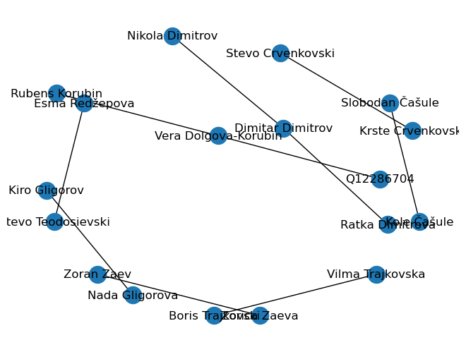
The graph doesn’t look spectacular, but it show the possibilities of what can be achieved. The few data points we had actually helped having a readable graph like this. Probably a different visualization would be better suited if the relations were many.